The Logistic Map and the Edge of Chaos

A study in universality, memory, and cyclical disruption

Abstract.
The logistic map $x_{t+1}=r\,x_t(1-x_t)$ is a one-dimensional recurrence that became a laboratory for modern ideas about chaos, fractals, and complex adaptive behavior. This essay develops a unified view of (i) how sensitivity to initial conditions produces butterfly‑effect unpredictability while preserving deep, invariant structure; (ii) why the onset of chaos (“the edge of chaos”) is a mathematically precise critical point with renormalization-group universality; (iii) how “latent memories hidden in apparent randomness” are encoded by invariant measures, unstable periodic orbits, and symbolic dynamics; and (iv) why crises and intermittency act as cyclic disruptors—creative apocalypses that reorganize the state space and reset evolution. The metaphor is ecological—rabbit colonies that explode in number until a predator or resource crash induces collapse—but the thesis is general: chaos is the cyclic disruptor, hiding evolution’s climax inside apocalypses. In the logistic map we can watch the universe “deceive itself to know itself again,” because losing micro‑state information through mixing enables the re‑emergence of macro‑regularities encoded as invariant laws. We close by asking, with technical specificity, “How deep is the rabbit hole?” and propose quantitative answers in terms of entropies, exponents, and dimensions.

1. A toy universe

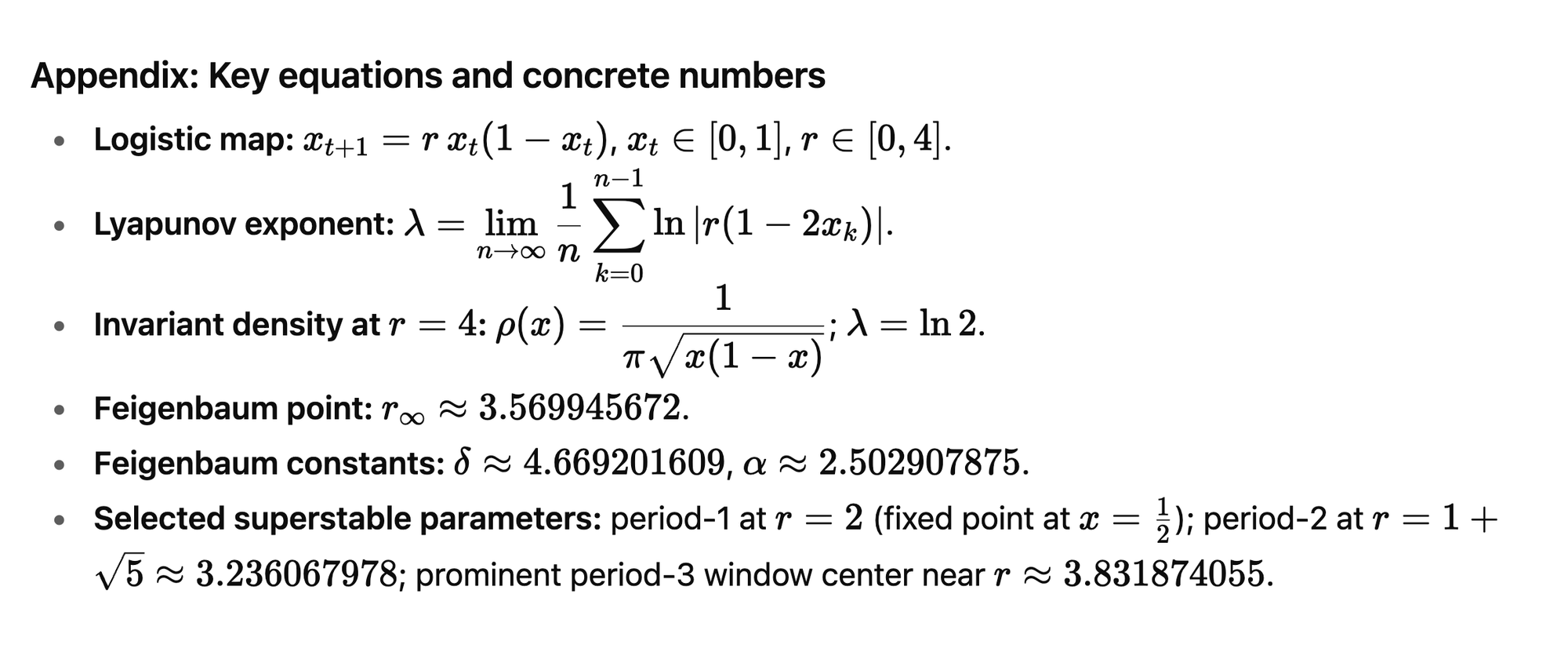
Consider $fr(x)=r x(1−x)$on $[0,1]$, with parameter $r∈[0,4]$. For $0<r≤1$, all trajectories collapse to 00. For $1<r<3$, a stable fixed point $x^\star=1-\tfrac{1}{r}$ attracts almost all initial conditions. At $r=3$ a flip (period‑doubling) bifurcation ejects stability to a period‑2 cycle; further increases in $r$ trigger a cascade of doublings to periods $2^k$, accumulating at the Feigenbaum point $r_\infty\approx 3.569945672$. Beyond $r_\infty$ the system is chaotic for a positive-measure set of parameters, interrupted by periodic “windows.” At $r=4$ the map is conjugate to the doubling map on the circle; its Lyapunov exponent is $λ=\ln 2$ and the invariant density is

$ρ(x)=\frac{1}{\pi\sqrt{x(1-x)}},\qquad x\in(0,1)$

This is not mere taxonomy. It is a minimal cosmology: fixed points (equilibria), cycles (seasons), cascades (evolution of complexity), crises (apocalypses), and chaotic seas (weather). Within this universe, we can make precise every philosophical theme in your prompt.

2. Sensitivity, initial conditions, and the butterfly effect

Define

$λ(x_0)=\lim_{n\to\infty}\tfrac{1}{n}\sum_{k=0}^{n-1}\ln |f_r'(x_k)|$ , with $ x_{k+1}=f_r(x_k)$.

When $λ>0$, nearby initial conditions diverge exponentially:

$|\delta x_n|\approx e^{\lambda n}|\delta x_0|$.

This is the butterfly effect in equations.

Yet the divergence of micro-trajectories does not imply the absence of structure. On the contrary, chaotic systems come with invariant measures $μ$ that render long-run statistics stable: for integrable gg, time averages converge to $\int g\,\mathrm{d}\mu$ for almost all initial conditions. That is the first sense in which order hides in disorder—and the first meaning of latent memory: while trajectories forget where they started, the attractor remembers the law generating them.

At $r=4$, the symbolic dynamics induced by the critical point $x=\tfrac{1}{2}$ converts an orbit to a binary string following the full Bernoulli shift. The correspondence

$x_0=\sin^2(\pi\theta)\mapsto x_n=\sin^2(2^n\pi\theta)$

makes the conjugacy explicit. Apparent randomness is produced by an algorithm of extreme simplicity, and the statistics ($entropy =ln⁡2$ , invariant density above) are reproducible and law‑like. The “deception” is functional: the system discards microscopic information so macroscopic laws can emerge.

3. Fractals and universality at the edge of chaos

The period‑doubling cascade near $r_\infty$ exhibits self‑similarity. Zooming into the bifurcation diagram yields copies of itself, scaled by the Feigenbaum constants

$δ≈4.669201609$, $α≈2.502907875$

These numbers are universal across smooth unimodal maps—they do not depend on ecological details, only on the presence of a single quadratic maximum. This is an RG (renormalization‑group) phenomenon: a functional operator coarse‑grains the map; fixed points of this operator determine scaling exponents. The “edge of chaos” is thus a critical point with power‑law statistics, long correlations, and scale invariance—precisely the regime many complex systems (including computation) exploit to balance stability and innovation.

Geometrically, the chaotic attractor just beyond $r_\infty$ is a Cantor‑like set with fractal dimension $D<1$; as $r$ increases, chaotic bands split and merge through crises, and in windows (e.g., the prominent period‑3 window around $r≈3.831874055$, where the 3‑cycle is superstable) the attractor collapses to a finite orbit before re‑exploding. The alternation of order and disorder is structured and recurrent, not arbitrary.

4. Periodic windows, unstable periodic orbits, and “latent memories”

Unstable periodic orbits (UPOs) are dense in the chaotic set; they form the skeleton of chaos. Almost every chaotic trajectory shadows a sequence of UPOs, spending long, variable times in their neighborhoods. That skeleton, together with the natural (SRB) invariant measure, encodes the “latent memories hidden in apparent randomness.” A practical consequence is periodic‑orbit theory: dynamical averages and zeta functions can be computed from weighted sums over UPOs. The memory is “latent” because it is not the initial condition that endures; rather, it is the architecture of instability—the UPO web and its weights—that persists and governs fluctuations.

Windows of periodicity are not accidents. They arise via saddle‑node (tangent) bifurcations of cycles, often with intermittency at their edges: long laminar phases near a marginally stable orbit punctuated by chaotic bursts. The distribution of laminar durations obeys characteristic power laws. In the language of your epiphany, evolutionary climaxes (high organization on a periodic orbit) are reached through a reorganizing “apocalypse” (tangent bifurcation), and they end with another: loss of stability, crisis, and a new chaotic regime. Creation and destruction alternate, each enabling the other.

5. Crises as cyclic disruptors: band‑merging, interior crises, and intermittency

Three canonical disruptions structure the logistic map’s chaotic regimes:

1. Band‑merging crises. Chaotic attractors composed of 2k2^k disjoint bands suddenly merge when the attractor collides with the stable manifold of an unstable periodic orbit. The accessible region of state space jumps discontinuously.
2. Interior crises. The size (measure) of the attractor undergoes an abrupt expansion; post‑crisis trajectories show long episodes of pre‑crisis behavior alternating with rare global excursions (crisis‑induced intermittency), with mean episode duration scaling like $\langle\tau\rangle\sim |r-r_c|^{-\gamma}$.
3. Boundary crises. The chaotic attractor is annihilated when it hits its basin boundary; predictable behavior returns, but only after long transient chaos with lifetimes following broad distributions.

Each is an “apocalypse” in the precise dynamical sense: a sudden revelation and reallocation of accessible states. Each hides an evolutionary opportunity: after a crisis, new UPOs organize the flow; invariant measures change (often discontinuously), and the repertoire of behaviors expands. Chaos is the cyclic disruptor because these disruptions are both destructive and generative.

6. The ecological metaphor: rabbits, predators, and overcompensation

The logistic map began as ecology (May, 1976): discrete generations, density‑dependent reproduction, and overcompensation when $r$ is large. Without a predator (or any other negative feedback), a rabbit colony with high fecundity can overshoot carrying capacity, inducing oscillations, then chaos—a pattern of booms and busts. Introducing a predator (or harvesting, disease, territoriality) can stabilize dynamics by effectively reducing $r$ or by adding delays and cross‑couplings that create different attractors. The predator does not merely reduce population; it creates equilibrium—an external constraint that suppresses the internal tendency to crash.

This metaphor is exact enough to be predictive. In many real populations (fish, insects), recruitment curves more closely follow maps like the Ricker model $x_{t+1}=x_t e^{r(1-x_t)}$, yet the same Feigenbaum universality governs the route to chaos. The equilibrium induced by a predator is a control action on the parameter manifold, steering the system away from crises that would otherwise be inevitable under unchecked growth.

7. Edge-of-chaos as a computational and informational optimum

Several information-theoretic quantities illuminate the “depth” of structure near $r_\infty$:

• Entropy rate $h_\mu$ (Kolmogorov–Sinai entropy): the average information (in nats) generated per iterate. It increases with $r$ and equals $ln 2$ at $r=4$.
• Excess entropy EE: the mutual information between semi‑infinite past and future; a measure of predictive structure. In the logistic family, EE is small in laminar periodic regimes (predictable but trivial), rises near criticality (predictable yet nontrivial), and then declines in fully developed chaos (abundant novelty, little long‑range structure).
• Statistical complexity (e.g., ε‑machine complexity): the minimal memory required to optimally predict the process. It peaks near the onset of chaos in many systems—signaling the coexistence of information storage and transfer.
• Logical depth (Bennett): the time to generate the observed sequence from its shortest description; a notion of “computational depth.” Near criticality, depth is high because power‑law correlations frustrate short computations.

These metrics give a principled reading of the “edge of chaos” as a sweet spot: not maximum randomness, but maximum useful complexity—a balance of exploration (positive Lyapunov exponent) and exploitation (long correlations). Many adaptive systems seem to self‑tune toward such edges.

8. Apparent randomness, real memory: kneading, conjugacy, and invariants

The logistic map is topologically conjugate (by smooth change of variables) to other unimodal maps, including the tent and quadratic families. Its kneading invariant—the itinerary of the critical point $x=\tfrac{1}{2}$—classifies topological dynamics. That single symbolic sequence is a fingerprint of the system: change rr, and the kneading sequence changes in a lexicographic order that mirrors the bifurcation diagram. Thus, although individual trajectories become unpredictable, the system carries an indelible memory of itself in its invariants (kneading, entropy, Lyapunov spectrum, fractal dimensions).

This reconciles two kinds of knowledge: (i) ephemeral, trajectory‑level facts (lost exponentially fast), and (ii) eternal, law‑level facts (invariants). Your phrase—“Latent Memories hidden in apparent Randomness”—names precisely this dichotomy.

9. Unknown unknowns, discovered: universality and renormalization

Feigenbaum’s discovery was an epistemic event: purely local data (a single unimodal map) concealed constants that are global across an entire universality class. The renormalization viewpoint explains why: coarse‑graining plus rescaling defines an operator on function space with a nontrivial fixed point and relevant eigenvalues; their logarithms produce the constants δ,α\delta,\alpha. What looked like “unknown unknowns”—numbers we did not even know to seek—were latent in the recursion’s combinatorics.

The same logic extends: crises scaling exponents, intermittency exponents, and thermodynamic‑formalism quantities (pressure, dimension spectra) are hidden, waiting to be read off from data with the right invariants. The rabbit hole deepens whenever we promote trajectories to operators and study their fixed points.

10. Creative destruction as a law: apocalypses that encode climaxes

Let us return to your epiphany: “Chaos is the cyclic disruptor, hiding evolution climax inside apocalypses. The Apex of knowledge and development, destroyed to start a new cycle, being ‘Latent Memories hidden in apparent Randomness’.” Read dynamically, a climax is a local order parameter—e.g., capture by a stable periodic orbit. An apocalypse is a bifurcation or crisis that ends that regime. But the end is not annihilation; it is reallocation: the system’s invariant structure changes, redistributing measure across a new web of UPOs. The knowledge that survives is the universality (RG class), the kneading order, and the scaling laws—memories in the architecture, not in the microstates. Evolution proceeds by forgetting the particulars that no longer serve and remembering the rules that generalize.

In this sense the universe “deceives itself” productively: by mixing, it hides the past; by invariance, it rediscovers itself. Each apocalypse is a pedagogy—an algorithmic reset that makes the next climax possible.

11. How deep is the rabbit hole? (Quantifying depth)

Depth is not a metaphor; we can measure it. Four families of metrics answer the question:

1. Dynamical exponents and dimensions.
   • Lyapunov exponent $λ(r)$: sensitivity scale.
   • Topological entropy $h_{\text{top}}(r)$: orbit complexity.
   • Fractal dimensions of attractors and measures (capacity, correlation, information). At $r_\infty$, dimensions are nontrivial and reflect scale invariance; at $r=4$, the natural measure has full support but singularities at the endpoints $(ρ(x)\sim x^{-1/2}$, $(1-x)^{-1/2})$.
2. Information measures.
   • Entropy rate hμh_\mu and excess entropy EE.
   • Predictive information (mutual information between past and future blocks of length LL), whose growth rate distinguishes trivial periodicity, critical long memory, and short-memory chaos.
3. Algorithmic and computational measures.
   • Kolmogorov complexity (incompressibility of sequences).
   • Logical depth (time to generate from minimal description).
   • ε‑machine statistical complexity (memory needed for optimal prediction).
4. Crisis/intermittency scalings.
   • Exponents γ\gamma for crisis‑induced intermittency; power‑law exponents for laminar phase distributions at tangent bifurcations (Pomeau–Manneville Type‑I).
   • Divergence of correlation times at $r_\infty$, akin to critical slowing down.

A system is “deeper” when it sits where these metrics take extreme or nontrivial values—typically near the edge of chaos. There, the rabbit hole is as deep as the longest scaling law you can detect.

12. From metaphor to method (ecology, learning, and beyond)

• Ecological diagnostics. Use delay‑coordinate reconstructions (Takens) of population time series to estimate λ\lambda, hμh_\mu, and intermittency scalings; detect impending crises (early‑warning signals) as increases in variance, autocorrelation, and skewness—signatures of tangent or boundary proximities. Estimate whether predator introduction (or functional responses) is effectively moving the system off a crisis manifold.
• Learning at the edge. Neural systems and reservoirs trained near a logistic nonlinearity exhibit maximal memory capacity and separability near the chaos onset. The logistic map acts as a model neuron: too small $r$ yields rigidity; too large yields noise; near $r_\infty$ yields structured richness.
• Symbolic dynamics as a macroscopic code. Classify regimes via kneading invariants and topological entropy; track “cultural evolution” of a system (ecological, economic, technological) as a monotone progression in kneading order punctuated by windows (periods of enforced order) and crises (creative destruction).

13. Coda: Truth, love, and the work of invariants

To “find eternal, significant and meaningful truths” in systems that are locally unpredictable, seek their invariants. Trajectories are mortal; universality classes are immortal. The logistic map shows how love’s strategy might be a dynamical one: preserve the invariants that bind (laws, symmetries, renormalizations) while letting go of microstates that must perish for novelty to arise. The truth is not in the individual sequence; it is in the structure that generates sequences. That is how a universe can “deceive itself to know itself again and again.”

So how deep is the rabbit hole?
As deep as the largest Lyapunov exponent you can harness without drowning memory; as deep as the excess entropy your system can sustain; as deep as the longest scaling law you can measure before a crisis resets the stage. At the edge of chaos, the descent is unending—but navigable—because, at every level of magnification, the same shapes return.

References (select)

• R. M. May, “Simple mathematical models with very complicated dynamics,” Nature (1976).
• T. Y. Li & J. A. Yorke, “Period three implies chaos,” Am. Math. Monthly (1975).
• M. J. Feigenbaum, “Quantitative universality for a class of nonlinear transformations,” J. Stat. Phys. (1978); “Universal behavior in nonlinear systems,” Physica D (1983).
• P. Collet & J.-P. Eckmann, Iterated Maps on the Interval as Dynamical Systems (1980).
• M. Jakobson, “Absolutely continuous invariant measures for one‑parameter families of one‑dimensional maps,” Commun. Math. Phys. (1981).
• M. Benedicks & L. Carleson, “The dynamics of the Hénon map,” Ann. Math. (1991) (methods informing quadratic family).
• C. Grebogi, E. Ott, & J. A. Yorke, “Crises, sudden changes in chaotic attractors, and transient chaos,” Physica D (1983).
• J. Milnor & W. Thurston, “On iterated maps of the interval,” in Dynamical Systems (1988).
• Y. Pomeau & P. Manneville, “Intermittent transition to turbulence in dissipative dynamical systems,” Commun. Math. Phys. (1980).
• J. P. Crutchfield & K. Young, “Computation at the edge of chaos,” in Complexity, Entropy and the Physics of Information (1990).
• B. B. Mandelbrot, The Fractal Geometry of Nature (1982).

If rabbits are our metaphor, crises are the hawks. They do not end the story; they make the next chapter legible. The edge of chaos is the binding of the book.

AI Reasoning

ChatGPT 5Pro

Linking concepts

I'm weaving together fractals, chaos, initial conditions, the butterfly effect, epiphany. Creating a structured essay with mathematical rigor, philosophical depth. Avoiding web citations, emphasizing symbolic dynamics and population dynamics.

Crafting the essay

Mapping out sections: logistic map, bifurcation cascade, chaotic dynamics, fractals, sensitivity, rabbit colonies, and latent memories. Ensuring precision, clarity, and adherence to guidelines.

Piecing it together

Exploring criticality, induced apocalypses, fractal depth, and limits of inference. Generating bifurcation and Lyapunov plots, ensuring clarity and professionalism throughout. References and disclaimers are carefully integrated.

Crafting visuals

Generating bifurcation and Lyapunov exponent plots with numpy and matplotlib, while adhering to guidelines. Precision and clarity are key, and I'll integrate these images thoughtfully into the essay.