An illustrated explanation of Entanglement, The Mermin Device and Bells Inequality.

A source sends two particles to distant detectors. Each detector offers three settings and gives one of two results. The surprising part is the pattern across many trials: quantum mechanics predicts a pattern that no model based on independent local responses to shared instructions can reproduce.

The mathematical result and its experimental violation are well established. The remaining mystery concerns the physical account of the correlations and the emergence of definite measurement outcomes. We will build the counting argument first, then examine entanglement and the spin and photon apparatuses.

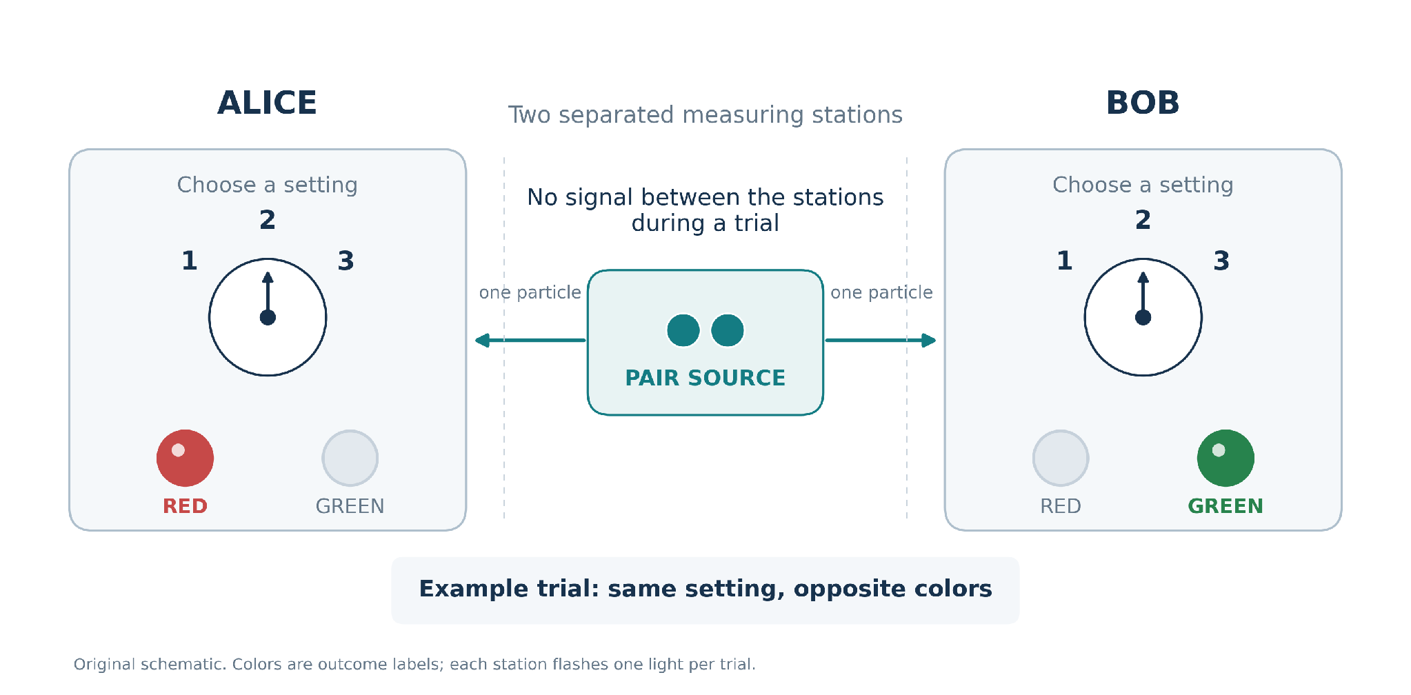
Figure 1. An original schematic of the Mermin device. Both detectors are set to 2 in this example, and their colours are opposite. Only one light flashes at each detector on a trial.

How to run a trial

Alice selects setting 1, 2, or 3 on the left. Bob makes the same kind of choice on the right. The source emits a pair, and each detector records either red or green. The observers later compare the settings and colours in their records. Red and green are labels for outcomes; they are not the colours of the particles.

Choose the settings independently and uniformly. Each of the nine ordered pairs, from 11 through 33, then has probability 1/9. This condition is essential to the overall percentages below.

Mermin’s original uses matching colours. Swap Bob’s red and green labels to convert between the conventions without changing the physics. [1, 2]

1 Why shared instructions seem sufficient

Perfect correlation by itself is familiar. Put a red card in one envelope and a green card in another. Mix the envelopes and send one to Alice and one to Bob. Each observer sees a random colour, but the colours always differ. Opening Alice’s envelope reveals what Bob will find because of the shared preparation.

The Mermin device adds a choice of test. A single card has only one answer. A local explanation of the device must provide a response to whichever of three settings is chosen, even if that choice occurs after the particles leave the source.

An instruction for every possible local setting

Suppose Alice’s particle carries the list RRG. This means red if her setting is 1, red if it is 2, and green if it is 3. To guarantee opposite colours whenever settings match, Bob’s corresponding list must be GGR. The detector reads only the entry for its chosen setting; no trial measures all three entries.

The list need not be written inside a particle. It represents any proposed underlying physical condition that fixes the local response. The source may distribute a different pair of lists on every trial. The argument gives that source unlimited shared randomness.

Count every possible setting pair

For this pair of lists, the table below shows the result for all nine choices. Alice’s setting identifies the row; Bob’s identifies the column. RG and GR count as opposite. RR and GG count as matching.

There are five opposite-colour cells: 11, 12, 21, 22, and 33. Because all cells are equally likely, this pair of instruction lists predicts opposite colours on 5/9 of trials. The other four cells predict matching colours.

The problem is already visible: 5/9 is about 55.6%, whereas the device’s overall quantum prediction is 50%. Could the source choose a better list?

2 The counting argument excludes every local list

A three-entry list has only eight possibilities. They fall into two classes. If all entries have one colour, its complementary list has the other colour at every setting, so all nine setting pairs give opposite results. If the list contains two entries of one colour and one of the other, five setting pairs give opposite results, as in the previous example.

The source may mix these cases in any proportions. An average of values that are all at least 5/9 cannot fall below 5/9. Therefore every such local instruction model satisfies this Bell inequality:

The inequality says at least, not strictly more than. The minimum is reached if the source uses only lists with two entries of one colour and one of the other.

The quantum prediction falls outside the bound

For the appropriate entangled pair, quantum mechanics predicts opposite colours with probability 1 at matching settings and probability 1/4 at each unequal setting pair. Three of the nine choices match and six differ, so:

Consider 900 trials with approximately 100 at each setting pair. Quantum mechanics predicts about 450 opposite results. A local instruction model satisfying the ideal matching-setting rule predicts at least 500 on average. These are expected counts, not exact requirements on every finite sample.

The difference is a reproducible statistical pattern. Nobody needs to predict an individual red or green result. Bell’s insight was that the broader explanation makes a testable numerical promise. The quantum pattern breaks that promise. [3]

We have used the ideal case of perfect opposite results at matching settings. Real experiments have noise and missed detections, so they use inequalities and statistical methods that account for those conditions. We return to that distinction in Section 8.

3 What a quantum measurement asks

To understand how quantum mechanics produces the pattern, first consider light. A photon is one quantum of the electromagnetic field. Its polarization concerns the direction of the field’s transverse electric component. The word transverse means perpendicular to the direction of travel. This description does not require imagining a photon as a little ball with an arrow painted on it.

An ideal polarization analyser set at a chosen angle distinguishes two perpendicular polarization outcomes. At a horizontal setting, those outcomes are horizontal H and vertical V. At a diagonal setting, they are D at 45° and A at 135°. The angle selects the question; the detector supplies an answer.

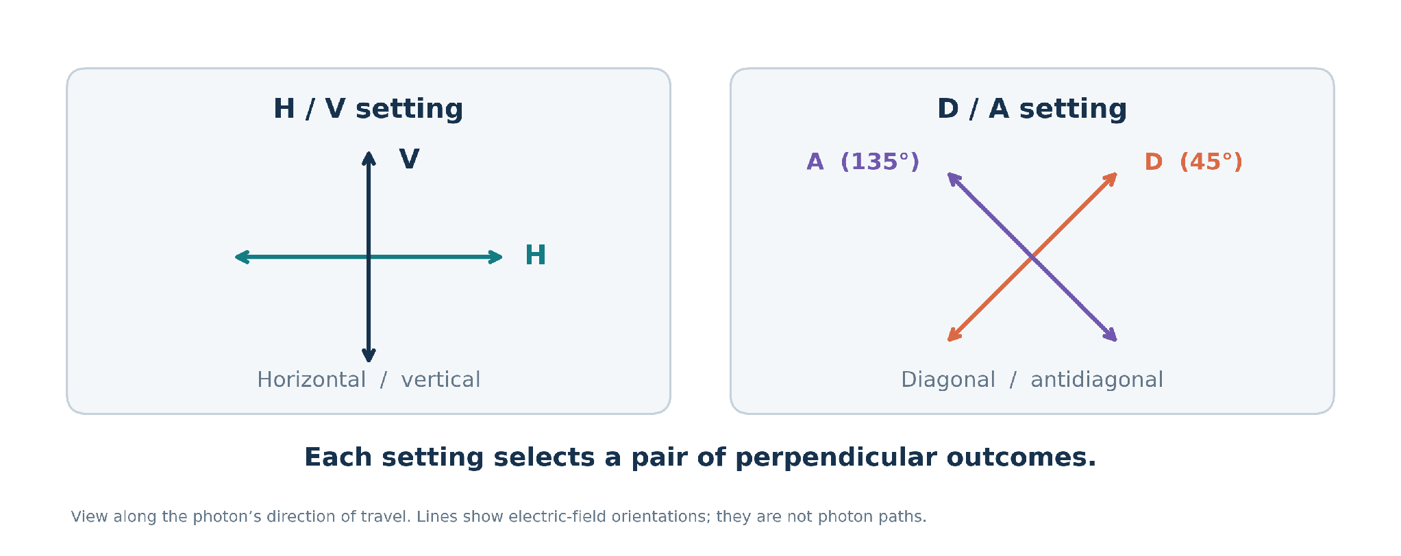
Figure 2. Two possible polarization measurement bases. H and V form one perpendicular pair; D and A form another. A basis specifies the alternatives distinguished by a measurement.

A state specifies probabilities for different tests

A photon prepared in H gives H with certainty in the H/V test. In the D/A test, it gives D or A with probability 1/2 each. The same preparation therefore has different outcome probabilities for different questions. A quantum state lets us calculate these probabilities.

A superposition combines probability amplitudes for alternative outcomes. Amplitudes are mathematical quantities whose contributions can reinforce or cancel. To find a probability, first combine amplitudes for indistinguishable alternatives, then take the squared magnitude of the total. Ordinary probabilities cannot cancel in this way.

The notation |H⟩ names the H quantum state. A bracket of this form is called a ket. For a pair, |HH⟩ refers first to Alice’s photon and then to Bob’s. A plus sign between kets combines amplitudes; it does not say that the source tosses a coin and prepares one listed possibility.

The entangled photon state

The factor 1/√2 makes the total probability equal to 1. Measuring this state in H/V gives HH or VV, each with probability 1/2. Each photon separately gives H or V at random, while their joint results always match.

For a pure joint state such as this one, entanglement means that the state cannot be written as a product of separate pure states for the two photons. Each photon still has a valid individual description: a mixed state that predicts its local statistics. The full pair contains information that those separate descriptions do not capture.

4 Why entanglement exceeds ordinary correlation

A classical preparation could produce HH on half the trials and VV on the other half. It would reproduce the entangled pair’s H/V results. Measuring only H/V would therefore leave us unable to distinguish the two preparations.

Rotate both analysers to the diagonal basis. Each H photon and each V photon gives D or A with equal probability. In the classical mixture, the separate photon states give four equally likely joint outcomes: DD, DA, AD, and AA. The results now match only half the time.

The coherent entangled state behaves differently. It always gives matching diagonal results. The reason is interference between the amplitudes associated with HH and VV. Here is the calculation, with every symbol introduced on the previous page.

Replace each H and V in the pair state using these expressions. The HH term contributes DD, DA, AD, and AA with positive signs. The VV term contributes DD and AA with positive signs but DA and AD with negative signs. When the two amplitudes are added, DA and AD cancel. DD and AA remain:

For example, the HH contribution to a DA result has amplitude +1/(2√2), while the VV contribution has amplitude −1/(2√2). Their sum is zero. In a classical mixture, we would instead add the positive probabilities from the two preparations; they would total 1/4.

Thus “the pair is HH or VV and we simply do not know which” describes a different physical preparation. Coherence has consequences that a rotated measurement can reveal.

This example rejects that particular mixture. Matching results in two bases alone do not establish the full Bell argument: a more elaborate local instruction model could imitate those limited data. Bell inequalities test the wider pattern across different choices on the two sides.

For general mixed states, the precise definition is broader: a state is entangled if it cannot be represented as a probabilistic mixture of product states. A correlated mixture can fail to factorize and still be unentangled. Entanglement and violation of a particular Bell inequality are also distinct: noise can leave entanglement present without a violation in that test. [5]

5 The spin apparatus behind the Mermin device

Spin is intrinsic angular momentum, with associated magnetic behaviour. It is not the literal rotation of a tiny solid sphere. For a spin 1/2 system, an ideal measurement along any selected axis has two outcomes, conventionally written + and −, corresponding to angular momentum components +ℏ/2 and −ℏ/2. The symbol ℏ is Planck’s constant divided by 2π.

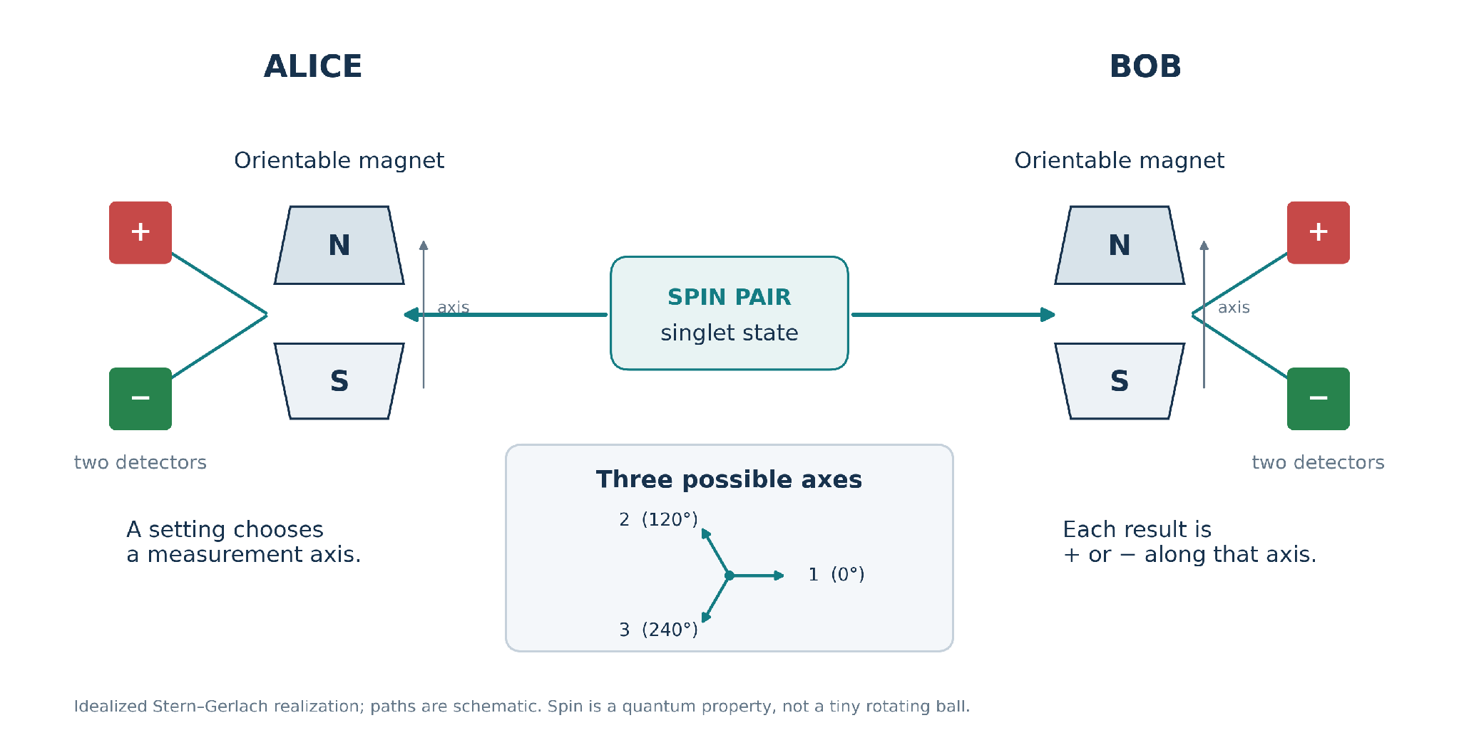
Figure 3. An idealized spin realization. An inhomogeneous magnetic field separates two spin outcomes. Rotating the analyser selects its measurement axis. The three directed axes are separated by 120°. This is a conceptual apparatus, not a diagram of an actual loophole-free experiment.

A Stern–Gerlach analyser sorts suitable neutral atoms through their magnetic interaction with a field that varies across the beam. The silver-atom demonstration illustrates the two-way splitting; it is not itself a source of entangled pairs. The Mermin realization additionally requires preparation of a suitable pair in a spin singlet state.

The arrows refer to outcomes along a reference axis. The singlet has total spin zero and predicts opposite outcomes whenever both analysers use the same axis. Neither individual outcome is fixed by the quantum state. At both wings, assign red to + and green to −.

For two axes separated by angle θ, the singlet predicts:

Use directed axes at 0°, 120°, and 240°. A matching pair has θ = 0°, giving probability 1. Every different pair has cosine θ = −1/2, giving probability 1/4. These are exactly the numbers used in the counting argument. A 240° directed difference has the same cosine as 120°.

6 The photon apparatus

A 2002 undergraduate experiment by Dietrich Dehlinger and M. W. Mitchell. The apparatus produces polarization-entangled photons rather than spin-entangled atoms. The schematic below reconstructs its principal components. [6, 7]

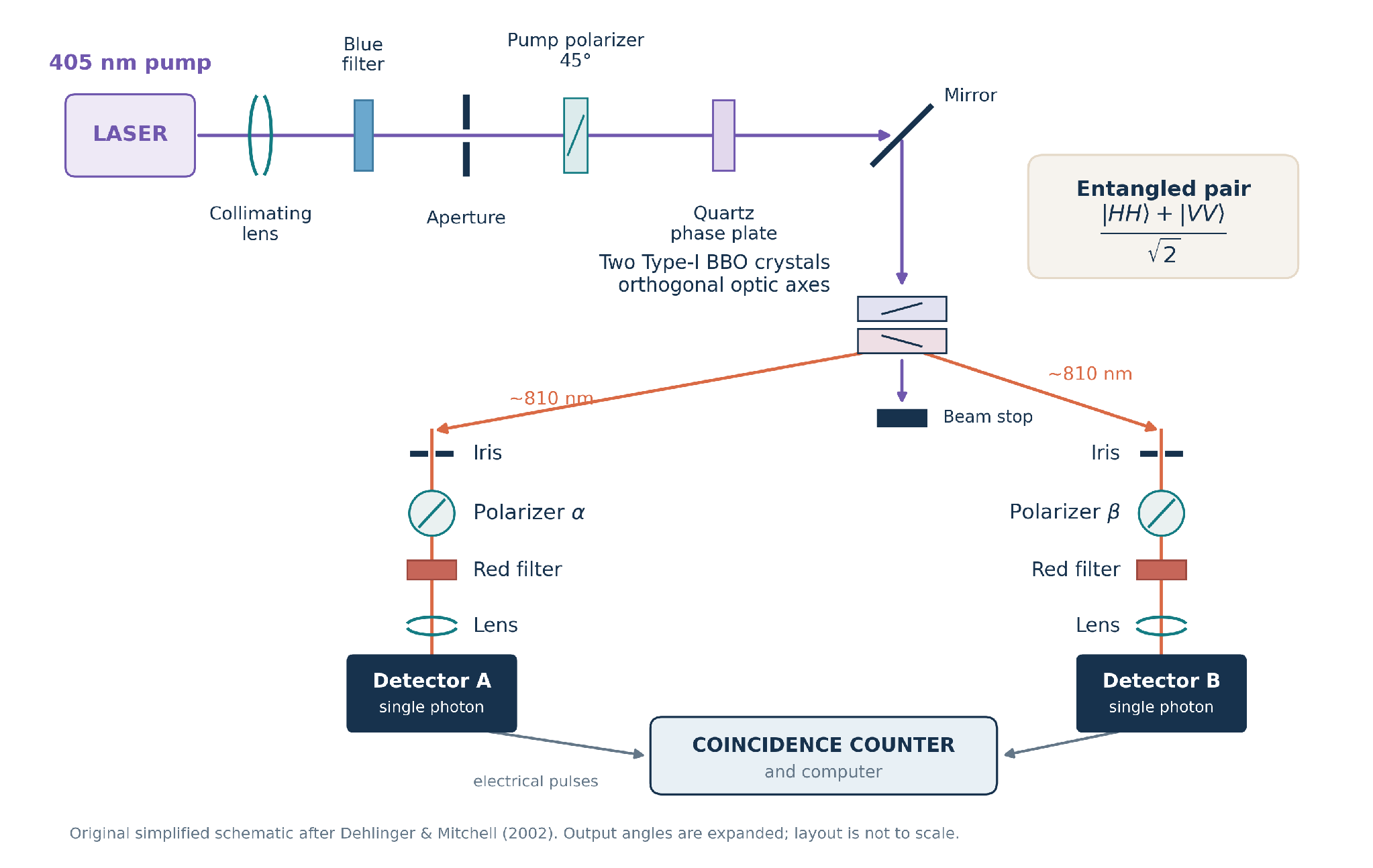
Figure 4. Reconstruction of the Dehlinger–Mitchell apparatus. This original schematic simplifies and expands the optical paths. It shows one transmitted-output detector per arm.

How the source creates a coherent pair

A violet laser supplies pump photons near 405 nanometres. Preparation optics set the pump polarization and relative phase. Two thin nonlinear crystals, made of beta barium borate or BBO, have perpendicular orientations. In a rare event called spontaneous parametric downconversion, the pump supplies energy for creation of a pair. Near equal energy sharing, each output photon has wavelength near 810 nanometres.

One crystal supplies an HH alternative, and the other supplies a VV alternative. When the two alternatives are indistinguishable in the relevant spatial, spectral, and temporal degrees of freedom, and their phase is controlled, their amplitudes combine coherently. Suitable preparation yields the Φ+ state introduced earlier. The source creates the joint state before the photons separate; separation does not erase it.

How the apparatus records correlations

Each arm has an aperture, a rotatable polarizer, a filter to reject stray pump light, focusing optics, and a single-photon detector. Detector pulses go to coincidence electronics. Nearly coincident clicks identify candidate pairs against background counts, and a computer records their rate.

The rotatable polarizers select the tests. The electronic coincidence comparison collects records from both arms after detection. It does not send information between the photons to generate their measurement outcomes.

Pair production alone does not guarantee polarization entanglement. Here it requires coherence between the HH and VV production alternatives.

7 Connecting photon results to the coloured lights

For the ideal Φ+ photon state, matching linear analyser angles produce matching physical polarization outcomes. The spin singlet gives opposite spin outcomes. Reversing Bob’s colour labels connects the two descriptions:

With this reversal at Bob’s display, matching physical outcomes become opposite colours. If α and β are the two polarizer angles, the photon state predicts:

To see why, suppose Alice obtains the outcome parallel to α. Bob’s conditional polarization is then parallel to α. Resolving that direction into Bob’s parallel and perpendicular directions gives amplitudes cos(α − β) and sin(α − β). Squaring them gives the probabilities. Alice’s perpendicular outcome gives the same probability for a matching result.

That is also the probability of opposite displayed colours under the reversed labels. Choose polarizer angles 0°, 60°, and 120°. Matching choices give probability 1. Different choices give cos²60° or cos²120°, both equal to 1/4. The nine-choice average is again 1/2.

The spin and photon angle rules differ. Spin uses cos²(θ/2); these linear polarization measurements use cos²(α − β). A polarization axis repeats after 180°, and its corresponding two-state measurement direction rotates through twice the physical analyser angle. Thus a 60° polarizer rotation supplies the correlation associated with a 120° spin-axis separation.

The teaching experiment tests a related inequality

The 2002 apparatus uses one detector per arm to measure transmitted photons. It estimates complementary outcomes in separate acquisition periods with a polarizer turned through 90°. A missing click alone is not a recorded second outcome: a photon may have been blocked, lost, or missed. An ideal analyser with two monitored outputs would more literally implement the two-light box.

The authors test the CHSH inequality, named after Clauser, Horne, Shimony, and Holt. It uses two settings per side. Assign +1 and −1 to the two physical polarization outcomes, using the same convention at both wings. Define E as the average product of their values: probability of matching outcomes minus probability of different outcomes.

For Φ+, E = cos[2(α − β)]. Using Alice’s angles 0° and 45°, and Bob’s 22.5° and −22.5°, gives three correlations +1/√2 and one −1/√2. Hence S = 2√2, about 2.828, above the local bound 2. The paper reports S = 2.307 ± 0.035 under its experimental assumptions. This is a CHSH result, not a measured 5/9 Mermin test. [6]

8 What assumptions a Bell test examines

The instruction-list proof is a compact example of a more general question. Can shared conditions from the past explain all the observed outcomes if each detector responds only to its own setting and those shared conditions?

A local common cause model

Let λ, pronounced lambda, denote the complete underlying information relevant to a trial. It may include details of the pair, the source, the detectors, and shared randomness. Let x and y denote Alice’s and Bob’s settings. Let A and B denote their outcomes. A Bell local model has this form:

The function ρ, pronounced rho, gives the probability distribution of λ. Each local response may itself be probabilistic. The product says that after λ is specified, neither the distant setting nor the distant outcome adds anything to the local response probabilities. Averaging over λ restores the correlations produced by shared preparation.

The model also assumes measurement independence: the distribution of λ is the same for each selected setting pair. This is a statistical independence condition, not a mathematical claim about human free will. A source whose hidden state were correlated with future setting choices would require a different analysis.

Why adding local randomness does not rescue the lists

Local random choices can be included in a more complete λ, producing a distribution over deterministic response tables. In this ideal example, perfect opposite outcomes at every matching setting make the point stronger: under the product rule, any λ that allowed the same colour on both sides would give a positive chance of a forbidden result. Therefore the relevant responses must be deterministic and complementary at each matching setting.

The lists are consequently a representation of the local model, not an arbitrary restriction to eight tiny computers. If a hidden theory changes its response according to the distant setting, or correlates λ with the settings, it has changed a premise. Bell inequalities apply to local stochastic models as well as deterministic ones. [3, 5]

How experiments make the ideal question testable

Real instruments miss particles, suffer noise, and cannot establish perfect correlations with finite data. A rigorous test must specify its trial rules and setting probabilities, handle nondetections appropriately, and assess statistical evidence against the local bound. Applying the simple 5/9 bound despite mismatches at identical settings would be invalid.

The undergraduate apparatus relies on sampling and stability assumptions and does not arrange rapid, spacelike separated choices. Independent experiments in 2015 closed the major detection and locality loopholes together, using entangled electron spins and entangled photons. “Loophole-free” is standard shorthand for that achievement; it does not establish every imaginable assumption without qualification. [8–10]

9 Why entanglement cannot send a faster than light message

Suppose Alice and Bob use the same H/V basis on a Φ+ pair. If Alice sees H, she can predict that Bob sees H. But Alice cannot choose H rather than V. Before her outcome is known to Bob, his own possibilities remain equally likely.

The second and third rows concern selected subgroups defined by Alice’s result. Bob cannot identify those subgroups from his local records. He must receive Alice’s record through an ordinary communication channel. Conditional certainty therefore does not supply a controllable signal.

For a spin singlet, the complete joint probability has a particularly simple form. Encode its two outcomes as +1 and −1:

To obtain Bob’s local probability, sum over both possible outcomes at Alice. The positive and negative terms cancel:

Changing Alice’s setting changes joint correlations but leaves Bob’s distribution at 1/2 for each outcome. Ignoring her result, her measurement also leaves his reduced state unchanged. This is no-signalling. Alice may sort her records afterwards, but cannot force Bob into a subgroup of her choice.

Why no signalling does not settle Bell locality

Bell locality is a stronger condition. It requires that an appropriate shared past explanation screen off the distant setting and result. Quantum mechanics preserves local no-signalling while producing a joint distribution that does not fit the Bell local model. These are different demands on an explanation.

What relativity adds

Two measurements are spacelike separated when light cannot travel from either measurement event to the other in the available time. Different inertial observers can then disagree about which event occurred first. A story in which Alice’s measurement physically acted first cannot be inferred as a frame-independent mechanism from the correlations.

The standard quantum calculation gives the same joint probabilities regardless of the order assigned to these separated local measurements. In mathematical terms, their measurement operators act on separate subsystems and commute. The data support the correlations and no-signalling; they do not establish that a collapse signal travelled instantaneously in a particular frame. [5]

10 The result that is settled and the questions that remain

Bell’s inequality is a proven constraint on a specified class of models. Experimental violations establish that the observed world cannot be explained by that class under the tested independence and experimental assumptions. The open questions concern the underlying physical picture.

The Einstein Podolsky Rosen concern

In 1935, Einstein, Podolsky, and Rosen argued that if one can predict a property of a distant system with certainty without disturbing it, that property should count as an element of reality. Their original example used position and momentum. The spin version makes the same tension easier to see: Alice may choose an axis and predict the corresponding result for Bob.

If a distant choice and measurement cannot affect Bob’s physical situation, it seems that his answer must already be available for whichever axis Alice selects. Quantum mechanics does not supply simultaneous definite answers for all those incompatible tests. EPR therefore challenged the completeness of the quantum description. Bell later showed that supplementing it with a local answer scheme creates statistical predictions that quantum mechanics can violate. [4]

Bell does not prove that reality disappears

The phrase “realism is false” compresses too much. Bell tests reject a conjunction of precise assumptions. They do not prove that every object lacks properties before measurement, that all hidden-variable accounts are impossible, or that determinism is impossible. A theory can preserve some definite underlying properties while abandoning Bell local causality.

A counterfactual result is the answer to a measurement that could have been performed but was not. Bell’s theorem rules out the relevant local, setting-independent response model. It does not by itself select a unique metaphysical conclusion about all unperformed measurements.

The separate measurement problem

Quantum theory’s usual evolution preserves superpositions. If a detector is treated as another quantum system, a pair superposition becomes a superposition correlated with detector records. Schematically:

Each term contains a definite-looking record, but the total state contains both alternatives. A person experiences a definite result. How should we connect that experience to the state and its evolution? This is the measurement problem. It would arise for a single detector as well; Bell’s theorem exposes a further constraint when separated systems are involved.

Decoherence explains why interaction with the environment suppresses observable interference between different macroscopic records. It helps explain the stability of a detector reading and the appearance of classical behaviour. Its significance for a unique outcome still depends on the interpretation adopted. [14]

11 Different accounts pay different explanatory costs

Several approaches reproduce the familiar Bell correlations while making different claims about physical reality. Bell data alone do not choose among accounts with the same predictions. The following are explanatory options, not additional findings established by the device.

State update without a detailed collapse mechanism

In operational use, the state predicts measurement statistics and is updated after an outcome to give conditional predictions. This calculates all the probabilities discussed here. It leaves open whether the update describes a physical event, a change in information, or something else; it does not specify an underlying mechanism.

Definite configurations with nonlocal dynamics

In de Broglie–Bohm type theories, particles have definite configurations guided by a quantum state. Entangled guidance depends on the whole configuration, making the dynamics nonlocal in the Bell sense. Standard equilibrium predictions reproduce quantum statistics. Bell violation therefore does not refute determinism or every form of realism. Reconciling this underlying description with relativistic structure raises further questions. [11]

Universal evolution and relative outcomes

Everett’s approach keeps the state evolving without fundamental collapse. Measurement correlates the system, apparatus, and observers. Definite records belong to branches or relative states of that joint description. Decoherence helps explain their practical independence. Questions about probability and branching remain; this does not recover the local single-outcome instruction model tested above. [12, 14]

A physical collapse law

Objective collapse theories modify quantum evolution so that definite outcomes emerge through physical stochastic processes. They can depart from standard predictions in other regimes, inviting further experiments. GRW is an important example. Existing Bell violations do not select a unique collapse model, nor make collapse a controllable message between the wings. [13]

Changing the independence assumption

Other proposals explore correlations between hidden conditions and measurement settings, or descriptions in which future boundary conditions help constrain past variables. These change the premises behind the local bound. A successful proposal must give a clear model and account for the observed statistical regularities; naming a relaxed premise is not yet an explanation of the apparatus.

The explanatory proposal

An account based on conservation and the absence of a preferred reference frame. Total angular momentum conservation remains exact. Different analyser axes measure different components, so their two results need not sum to zero. The relevant average relation says that, given Alice’s ±1 result, Bob’s mean result is −A cosθ. This relates quantized outcomes to the expected projection. [15]

Rotating an analyser changes its question; all three settings can occur within one laboratory inertial frame. The proposal offers a physical rationale for the correlations. Bell violation alone neither derives the postulates of special relativity nor uniquely resolves the interpretive questions. Conservation still supplies no local list of answers for every axis.

12 A guide to the terms and the evidence

Three numbers to keep distinct

1 is the ideal probability of opposite displayed colours at matching settings. 1/4 is the corresponding probability at each different setting pair. 1/2 is the average across all nine equally likely setting pairs. The local model requires that last average to be at least 5/9.

If we examine only the six unequal-setting choices, the same contradiction reads: the ideal local model requires an opposite-colour probability of at least 1/3, whereas quantum mechanics predicts 1/4. This follows by removing the three matching-setting cells, which always contribute opposite outcomes, from the nine-cell count.

The directly accessible evidence consists of detector records and their correlations. Quantum states explain their probabilities with great precision. Interpretations address what those states and records imply about the underlying world. Keeping these levels distinct preserves both the force of Bell’s result and the real scope of the unresolved questions.

Sources and further reading

Bracketed numbers refer to the sources below. The arithmetic, worked tables, and explanatory schematics are developed in this document. A good reading order is Mermin for the puzzle, Dehlinger and Mitchell for the photon laboratory, and Bell or the Brunner review for the assumptions.

[1] W. M. Stuckey. Beyond the Dynamical Universe Episode 8 Quantum Mysteries for Anybody The Mermin Device. Physics & Reality with Prof Stuckey. https://www.youtube.com/watch?v=f7UtF6cbPlk

[2] N. David Mermin. Quantum Mysteries for Anyone. The Journal of Philosophy 78, 397–408 (1981). A companion presentation to Bringing home the atomic world Quantum mysteries for anybody, American Journal of Physics 49, 940–943 (1981). https://www.ringnebula.com/CosIG/28e-Mermin-Quantum-mysteries-for-anyone-1981.pdf

[3] John S. Bell. On the Einstein Podolsky Rosen paradox. Physics Physique Fizika 1, 195–200 (1964). Original theorem. https://doi.org/10.1103/PhysicsPhysiqueFizika.1.195

[4] Albert Einstein, Boris Podolsky, and Nathan Rosen. Can Quantum Mechanical Description of Physical Reality Be Considered Complete. Physical Review 47, 777–780 (1935). https://doi.org/10.1103/PhysRev.47.777

[5] Nicolas Brunner and colleagues. Bell nonlocality. Reviews of Modern Physics 86, 419–478 (2014). A technical review of local models, inequalities, experiments, and applications. https://arxiv.org/abs/1303.2849

[6] Dietrich Dehlinger and M. W. Mitchell. Entangled photons nonlocality and Bell inequalities in the undergraduate laboratory. American Journal of Physics 70, 903–910 (2002). The photon state, correlations, and reported CHSH result. https://arxiv.org/abs/quant-ph/0205171

[7] Dietrich Dehlinger and M. W. Mitchell. Entangled photon apparatus for the undergraduate laboratory. American Journal of Physics 70, 898–902 (2002). Construction and operation of the apparatus. https://arxiv.org/abs/quant-ph/0205172

[8] B. Hensen and colleagues. Loophole free Bell inequality violation using electron spins separated by 1.3 kilometres. Nature 526, 682–686 (2015). https://arxiv.org/abs/1508.05949

[9] Marissa Giustina and colleagues. Significant loophole free test of Bell’s theorem with entangled photons. Physical Review Letters 115, 250401 (2015). https://arxiv.org/abs/1511.03190

[10] Lynden K. Shalm and colleagues. Strong loophole free test of local realism. Physical Review Letters 115, 250402 (2015). https://arxiv.org/abs/1511.03189

[11] David Bohm. A Suggested Interpretation of the Quantum Theory in Terms of Hidden Variables I and II. Physical Review 85, 166–179 and 180–193 (1952). https://doi.org/10.1103/PhysRev.85.166

[12] Hugh Everett III. Relative State Formulation of Quantum Mechanics. Reviews of Modern Physics 29, 454–462 (1957). https://doi.org/10.1103/RevModPhys.29.454

[13] G. C. Ghirardi, A. Rimini, and T. Weber. Unified dynamics for microscopic and macroscopic systems. Physical Review D 34, 470–491 (1986). https://doi.org/10.1103/PhysRevD.34.470

[14] W. H. Zurek. Decoherence einselection and the quantum origins of the classical. Reviews of Modern Physics 75, 715–775 (2003). https://arxiv.org/abs/quant-ph/0105127

[15] W. M. Stuckey, T. McDevitt, M. Silberstein, and T. D. Le. Answering Mermin’s challenge with conservation per no preferred reference frame. Scientific Reports 10, 15771 (2020). https://arxiv.org/abs/1809.08231

Eduardo Bergel and ChagGPT Astra

t333t.com Research